
Continuum Mechanics With Maple:
Mass, Momentum, Energy and Entropy, and Derivation of Constitutive Relations for Various Materials
This worksheet uses continuum mechanics principles to derive the laws governing flow behavior of elastic and viscous.
Pawan S. Takhar
Professor
Food Science and Human Nutrition
University of Illinois at Urbana-Champaign
(ptakhar@illinois.edu)
Copyright
The ContMech maple worksheet has all rights reserved to the author. The worksheet is provided as is, without guarantee of support or maintenance. The author is not liable for any damages resulting in any way from its use. Everyone is granted permission to copy, modify and redistribute this worksheet at no charge, provided due credit is given to the original developer in citations, references etc and the use is for academic purpose only. Commercial use or sale of this material in any form is strictly prohibited. This copyright notice should not be removed from the modified versions.
Introduction
This worksheet demonstrates the use of continuum mechanics framework for deriving constitutive equations for various materials. The constitutive relations can further be incorporated into balance laws to obtain laws like Fourier's law of heat transfer, Navier-Stokes equation of fluid flow, Hooke's law for elastic materials, stress-strain relations for viscoelastic materials etc. Although, , these engineering laws have been discovered through theoretical and experimental research spanning several decades, it can be demonstrated that by knowing the basic dependency relations, these can be obtained using the framework of continuum mechanics in a straightforward manner. Once the basic procedure is understood, one can play with dependent and independent variables in Constitutive Theory section of different materials to obtain new types of laws. For example, one can derive relations for studying the interaction of viscoelastic polymers with surrounding fluids.
The purpose of this worksheet is to demonstrate the use of continuum mechanics framework to students in science and engineering. I have tried to adhere to the notation used in classical textbook "Mechanics of Continua" by A.C. Eringen. Thanks to Maplesoft for adding Einstein's summation-convention based tensorial capabilities starting release 11, which made this work possible.
Notes
1) Eulerian and Lagrangian coordinates are indicated by vectors, X and Y, respectively. X=(x1,x2,x3) and Y=(y1,y2,y3).
2) Continuum mechanics literature uses capital indices for Lagrangian coordinates and small indices for Eulerian coordinates. However, in current version of Physics package, this type of use is not clearly described. Therefore, I will use c, i, j, k and l for Eulerian, and p, q, r and s for Lagrangian indices. In future Maple releases, if mixing of small and capital indices in single equations is allowed, I may update this worksheet.
2) Equations are in Cartesian coordinates, where the metric, Gij=δij(Kronecker Delta), and the components of the Christoffel symbols vanish.
3) Transformation between Eulerian and Lagrangian coordinates is denoted by function X=f(Y) or X=f(y1, y2, y3). It could have been denoted by X=X(Y) but the current version of Physics package does not allow this type of relation (see my blog on Mapleprimes).
Nomenclature
X (Eulerian coordinates), Y (Lagrangian coordinates), rho (density), v (velocity), sigma (stress tensor), E (Lagrangian strain tensor), d (deformation tensor), Mu (Generalized coefficient of viscosity), Nu (shear viscosity for isotropic fluids), lambda (dilational viscosity for isotropic fluids).
pi (thermodynamic pressure), Q (surface heat flux), H (body source of heat), epsilon (internal energy density), A (Helmholtz free energy), b (body source of entropy), S (surface flux of entropy), bf (body force), theta (temperature), eta (entropy), f (X=f(Y), function relating Eulerian and Lagrangian coordinates), md (Material time derivative), Md (inert form of md).
Settings
restart;
with(PDEtools):
with(Physics):
>
Setup(coordinatesystems = {X, Y}, spacetimeindices=lowercaselatin,dimension = 3, differentiationvariables=X, signature = `+`);
![]()
![]()
![]()
![]()
![]()
![]()
(5.1)
Define Tensors
2D Tensors
Define(sigma, E, d, Mu,symmetric);
![]()
![]()
(6.1)
1D Tensors
Define(S, Q, bf,f, v);
![]()
![]()
(6.2)
Declarations and Operators
declare((rho,pi,sigma,d,Nu,lambda,S,Q,epsilon,A,bf,v,H,b,theta,eta)(X,t));
![]()
![]()
![]()
![]()
![]()
![]()
![]()
![]()
![]()
![]()
![]()
![]()
![]()
![]()
![]()
![]()
(7.1)
declare((E,f[i])(Y, t));
![]()
![]()
(7.2)
Material Time Derivative
md:=x->diff(x,t)+v[c]*d_[c](x);
![]()
(7.1.1)
Inert form of Material Derivative (Md)
alias(Md=%md):
Balance Equations
Mass Balance
eqb1:= Md(rho(X,t))+rho(X,t)*d[i,j](X,t)*KroneckerDelta[i,j] = 0;
![]()
(8.1.1)
Momentum Balance
eqb2:=d_[i](sigma[i,j](X,t))=-rho(X,t)*(bf[j](X,t)-Md(v[j](X,t)));
![]()
(8.2.1)
Energy Balance
eqb3:=-rho(X,t)*Md(epsilon(X,t))+sigma[i,j](X,t)*d[i,j](X,t)+d_[i](Q[i](X,t))+rho(X,t)*H(X,t)=0;
![]()
(8.3.1)
Entropy Inequality
Net production rate of entropy
eqee1:=rho(X,t)*Md(eta(X,t))-rho(X,t)*b(X,t)-d_[i](S[i](X,t))>=0;
![]()
(8.4.1)
Assuming, it is a simple thermomechanical process, the surface and body sources of entropy depend only on
eqm2:={S[i](X,t)=Q[i](X,t)/theta(X,t),b(X,t)=H(X,t)/theta(X,t)};
![]()
(8.4.2)
eqee2:=subs(eqm2,eqee1);
![]()
(8.4.3)
Substitute the energy equation (eqb5) into the above entropy inequality (eqee2) via "rho*H" term
eqb4:=H(X,t)=solve(eqb3,H(X,t));
![]()
(8.4.4)
eqee3:=subs(eqb4,eqee2);
![]()
(8.4.5)
eqee4 := expand(Simplify(eqee3));
![]()
(8.4.6)
Internal energy (ε) in the above equation is a function of entropy, which is difficult to measure. To make it a function of easily measurable, temperature, perform the Legendre transformation that relates Helmholtz free energy (A) to ε via is ε=A+θη.
Relation between epsilon and A:
eqm4:=epsilon(X,t)=A(X,t)+theta(X,t)*eta(X,t);
![]()
(8.4.7)
Take material time derivative of both sides:
eqm5:=Md(epsilon(X,t))=Md(A(X,t))+theta(X,t)*Md(eta(X,t))+eta(X,t)*Md(theta(X,t));
![]()
(8.4.8)
eqee5:=subs(eqm5,eqee4);
![]()
(8.4.9)
eqee6:=expand(simplify(eqee5));
![]()
(8.4.10)
Constitutive Theory: Elastic Materials
Up to the balance laws, number of variables are more than the number of equations. This is expected because while making the continuum assumption, the molecular scale information has been averaged out. This eliminated the information on nature of materials. To include nature of materials at the continuum scale, constitutive theory is formulated. First, let us formulate this theory for elastic materials.
eqEL1:=A(X,t)=fA(theta(X,t),E[i,j](Y,t));
![]()
(9.1)
Chain rule
eqEL2:=Md(A(X,t))=diff(fA(theta,E),theta)*Md(theta(X,t))+diff(fA(theta,E[r,s]),E[p,q])*md(E[p,q](Y,t));
![]()
(9.2)
eqEL3:=Simplify(eqEL2);
![]()
(9.3)
The following relation relates the Lagrangian strain tensor (E[p,q]) to the rate of deformation tensor d(k,l).
eqEL4:=md(E[r,s](Y,t),t)=d[i,j](X,t)*d_[r](f[i](Y,t),[Y])*d_[s](f[j](Y,t),[Y]);
![]()
(9.4)
Notice that on left hand side of previous equation, material derivative turns out to be equal to the partial time derivative. This is expected as E[p,q] is in Lagrangian coordinates. In Lagrangian coordinates, material derivative is equal to partial time derivative. The Lagrangian coordinates are indicated by capital indices and the variable "Y=(y1,y2,y3)".
eqEL5:=subs(eqEL4,eqEL3);
eqEL6:=subs(eqEL5,eqee6);
![]()
(9.5)
eqEL7:=collect(eqEL6, [d[i, j](X, t), Md(theta(X, t))]);
![]()
![]()
(9.6)
Imposing Restrictions Using Entropy Inequality to obtain Constitutive Relations for Elastic Materials
From constitutive equation (eqEL1) it can be concluded that coefficients of variables ![]() , Md(θ) and
, Md(θ) and ![]() in (eqEL7) are independent of these variables. Therefore, to satisfy the inequality these coefficients must be zero. This leads to non-equilibrium relations, which are satisfied both at and away from equilibrium.
in (eqEL7) are independent of these variables. Therefore, to satisfy the inequality these coefficients must be zero. This leads to non-equilibrium relations, which are satisfied both at and away from equilibrium.
Stress Equation
>
EqEL8:=sigma[i,j](X,t)=solve(op(1,rhs(eqEL7))=0,sigma[i,j](X,t));
![]()
(9.7)
This equation indicates that stress in an elastic material is proportional to derivative of Helmholtz free energy, w.r.t. the strain tensor (![]() ). This term is property of the material similar to coefficient of elasticity.
). This term is property of the material similar to coefficient of elasticity. ![]() depicts strain in the material.
depicts strain in the material.
Entropy Equation
>
eqEL9:=eta(X,t)=solve(op(2,rhs(eqEL7))=0,eta(X,t));
![]()
(9.8)
This indicates that entropy and temperature are related. They form a dual.
Heat Equation
>
eqEL10:=Q[i](X,t)=solve(op(3,rhs(eqEL7))=0,Q[i](X,t));
![]()
(9.9)
Since, thermal gradient was not considered in the constitutive equation for the elastic material, heat flux is zero.
Constitutive Theory: Viscous Fluids
Now, let us formulate the constitutive theory for viscous fluids.
eqVisc1a:=A(X,t)=fA(theta(X,t),rho(X,t),d[k,l](X,t));
![]()
(10.1)
Like A, other dependent variables, stress (σ) and heat flux (Q) are also considered to be a function of theta, rho and d[k,l].
eqVisc2a:=sigma[i,j](X,t)=fsigma[i,j](theta(X,t),rho(X,t),d[k,l](X,t));
![]()
(10.2)
eqVisc3a:=Q(X,t)=fQ(theta(X,t),rho(X,t),d[k,l](X,t));
![]()
(10.3)
Chain rule
eqVisc2:=Md(A(X,t))=diff(fA(theta,rho,d),theta)*Md(theta(X,t))+diff(fA(theta,rho,d),rho)*Md(rho(X,t))+diff(fA(theta,rho,d[g,h]),d[i,j])*md(d[i,j](X,t));
![]()
(10.4)
>
eqVisc3:=Simplify(eqVisc2);
![]()
(10.5)
eqVisc4:=subs(eqVisc3,eqee6);
![]()
![]()
(10.6)
In the next step, we mass solve balance equation (eqb1) and substitute the resulting Md(rho) value in eqVisc4. Direct substitution does not work, so we have aid Maple package by solving for Md(rho), before it is substituted in eqVisc4. This will eliminate Md(rho).
>
eqVisc5:=subs(Md(rho(X,t))=solve(eqb1,Md(rho(X,t))),eqVisc4);
![]()
![]()
(10.7)
>
eqVisc6:=collect(eqVisc5, [d[i,j](X,t),Md(theta(X, t))]);
![]()
![]()
(10.8)
Imposing Restrictions Using Entropy Inequality to obtain Constitutive Relations for Elastic Materials
Non-Equilibrium Relations
From constitutive equation (eqVisc1) it can be concluded that coefficients of variables Md(θ), Md(d[i, j]) and ![]() in (eqVisc6) are independent of these variables. Therefore, to satisfy the inequality these coefficients must be zero. This leads to non-equilibrium relations, which are satisfied both at and away from equilibrium.
in (eqVisc6) are independent of these variables. Therefore, to satisfy the inequality these coefficients must be zero. This leads to non-equilibrium relations, which are satisfied both at and away from equilibrium.
Helmholtz Free Energy-Deformation Rate Tensor Relation
Note in third term of Entropy inequality (eqVisc6) involves Md(d[i,j]). Coefficient of this variable is independent of Md(d[i,j]. Therefore to satisfy the entropy inequality, this coefficient must be zero.
>
eqVisc7:=diff(fA(theta,rho,d[g,h]),d[i,j])=0;
![]()
(10.1.1)
>
eqVisc8:=Simplify(eqVisc7);
![]()
(10.1.2)
Therefore, Helmholtz free energy, fA for viscous fluids is independent of the deformation rate tensor.
Entropy Equation
>
eqVisc9:=eta(X,t)=solve(op(2,rhs(eqVisc6))=0,eta(X,t));
![]()
(10.1.3)
This indicates that entropy and temperature are related. They form a dual.
Heat Equation
>
eqVisc10:=Q[i](X,t)=solve(op(4,rhs(eqVisc6))=0,Q[i](X,t));
![]()
(10.1.4)
Since, thermal gradient was not considered in the constitutive equation for the elastic material, heat flux is zero.
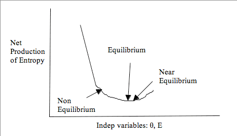
Equilibrium Relations
Stress Equation
>
eqVisc11:=sigma[i,j](X,t)=solve(op(1,rhs(eqVisc6))=0,sigma[i,j](X,t));
![]()
(10.2.1)
Let us define, thermodynamic pressure (π) as:
>
eqVisc12:=diff(fA(theta,rho,d),rho)=pi(X,t)/rho(X,t)^2;
![]()
(10.2.2)
>
eqVisc13:=subs(eqVisc12,eqVisc11);
![]()
(10.2.3)
Near-Equilibrium Results
Now let us derive near-equilibrium equation for stress. First, let us substitute the non-Equilibrium equations (eqVisc8, eqVisc9 and eqVisc10) in the entropy inequality (eqVisc6) to obtain the residual (non-zero) terms. Since, we have substituted non-equilibrium terms the resulting residual inequality will hold for processes both near and away from equilibrium.
eqVisc14:=subs({eqVisc8,eqVisc9,eqVisc10},eqVisc6);
![]()
(10.3.1)
eqVisc15:=subs(eqVisc12,eqVisc14);
![]()
(10.3.2)
>
eqVisc16:=collect(eqVisc15,{theta(X,t),d[i,j](X,t)});
![]()
(10.3.3)
In above equation, since the coefficient of d[i,j] is a function of d[i,j], it needs to be linearized around d[i,j] using Taylor series expansion to satisfy inequality for all independent processes. The first order expansion leads to:
eqVisc17:=op(1,rhs(eqVisc16))=Mu[i,j,k,l]*d[k,l](X,t);
![]()
(10.3.4)
eqVisc18:=sigma[i,j](X,t)=solve(eqVisc17,sigma[i,j](X,t));
![]()
(10.3.5)
The near-equilibrium equation is same as the classical equation for viscous flow. M[i,j,k,l] is generalized coefficient of viscosity for anisotropic fluids. For isotropic fluids, it has the form (Segel and Handelman, 1977):
eqVisc19:=Mu[i,j,k,l]=lambda*KroneckerDelta[i,j]*KroneckerDelta[k,l]+Nu*(KroneckerDelta[i,k]*KroneckerDelta[j,l]+KroneckerDelta[i,l]*KroneckerDelta[j,k]);
![]()
(10.3.6)
eqVisc20:=subs(eqVisc19,eqVisc18);
![]()
(10.3.7)
eqVisc21:=Simplify(eqVisc20);
![]()
(10.3.8)
This is the classical stress constitutive equation for both compressible and incompressible isotropic fluids.
Navier-Stokes Equation
By substituting the above stress-constitutive equation (eqVisc21) in the momentum balance equation (eqb2), one obtains the celebrated Navier-Stokes equation.
eqVisc22:=subs(eqVisc21,value(eqb2));
![]()
(10.3.1.1)
eqVisc23:={d[i,j](X,t)=1/2*(d_[i](v[j](X,t))+d_[j](v[i](X,t))),Simplify(d[k,l](X,t)*KroneckerDelta[k,l]=d_[k](v[k](X,t)))};
![]()
(10.3.1.2)
eqVisc24:=subs(eqVisc23,eqVisc22);
![]()
![]()
(10.3.1.3)
eqVisc25:=Simplify(%);
![]()
(10.3.1.4)
eqVisc26:=collect(eqVisc25,[d_[i](d_[j](v[i](X,t))),rho(X,t)]);
![]()
(10.3.1.5)
Here the square box represents the dAlembertian (or Laplacian ) operator ( ∇2v). This is the Navier-Stokes equation for compressible viscous fluids. Thus, we can obtain the Navier-Stokes equation using the framework of continuum mechanics by using general balance laws and constitutive knowledge of dependent and independent variables.
Summary
The framework of continuum mechanics allows deriving most engineering laws by using the general balance laws, knowledge of dependent and independent variables and imposing restrictions via entropy inequality. In this worksheet I demonstrate the procedure for obtaining equations for elastic and viscous materials. Once the procedure is understood, one can play with constitutive theory to obtain new types of resulting equations.
References
-Eringen, A. C. (1980). Mechanics of continua. Huntington, New York, U.S.A., R. E. Krieger Pub. Co.
-Segel, L. A. and G. H. Handelman (1977). Mathematics applied to continuum mechanics. New York, Macmillan.
-Singh (Takhar), P. P., J. H. Cushman, et al. (2003). "Thermomechanics of swelling biopolymeric systems." Transport in Porous Media 53(1): 1-24.